Reproducibility assessment data analysis for “Reproducible research and GIScience: an evaluation using GIScience conference papers”

This document visualises the expert assessment for accepted full papers at the GIScience conference series for the following conferences and proceedings.

• 2018: Tenth International Conference on Geographic Information Science, Melbourne, Australia

  Proceedings 10th International Conference on Geographic Information Science (GIScience 2018). 2018. In Winter, S., Griffin, A., Sester, M. (Eds.), LIPICS Vol. 114. ISBN 978-3-95977-083-5. http://www.dagstuhl.de/dagpub/978-3-95977-083-5

• 2016: Ninth International Conference on Geographic Information Science, Sep 27, 2016 - Sep 30, 2016, Montreal, Canada

  Geographic Information Science. 2016. In J. A. Miller, D. O’Sullivan, & N. Wiegand (Eds.), Lecture Notes in Computer Science. Springer International Publishing. https://doi.org/10.1007/978-3-319-45738-3

• 2014: Eighth International Conference on Geographic Information Science, Sep 24, 2014 - Sep 26, 2014, Vienna, Austria > Geographic Information Science. 2014. In M. Duckham, E. Pebesma, K. Stewart, & A. U. Frank (Eds.), Lecture Notes in Computer Science. Springer International Publishing. https://doi.org/10.1007/978-3-319-11593-1

• 2012: Seventh International Conference on Geographic Information Science, Sep 18, 2012 - Sep 21, 2012, Columbus, Ohio, USA > Geographic Information Science. 2012. In N. Xiao, M.-P. Kwan, M. F. Goodchild, & S. Shekhar (Eds.), Lecture Notes in Computer Science. Springer Berlin Heidelberg. https://doi.org/10.1007/978-3-642-33024-7

The analysis is based on the assessment first published in “Reproducible research and GIScience: an evaluation using AGILE conference papers” (https://doi.org/10.7717/peerj.5072), see https://github.com/nuest/reproducible-research-and-giscience.

Reproduce paper

To create the assessment result data and figures based on this document you can run the following commands in a new R session after completing the prerequisites with the original paper corpus data. If you have problems rendering the document you can execute each chunk independently in RStudio.

# Following code is not executed when document is created
require("knitr")
require("rmarkdown")
rmarkdown::render("giscience-reproducibility-assessment.Rmd")

Software dependencies and code

This document does not install the required R packages by default. You can run the script install.R to install all required dependencies on a new R installation, or use install.packages(..) to install missing R packages. This is not required if you use the Docker container provided by the authors.

source("install.R")

The plots and tables of survey data and evaluation use the packages ggplot2, knitr::kable(), huxtable, and kableExtra. Required libraries and runtime environment description are as follows.

library("tidyverse")
library("tidyr")
library("readr")
library("ggplot2")
library("reshape2")
library("ggthemes")
library("grid")
library("gridBase")
library("gridExtra")
library("kableExtra")
library("huxtable")
library("here")
library("googlesheets4")
library("patchwork")
library("knitr")
library("kableExtra")
library("ggalluvial")
library("ggfittext")

Load data

assessment_file <- here::here("results/paper_assessment.csv")
codebook_file <- here::here("results/codebook.csv")

The data is loaded from a collaborative spreadsheet using the googlesheets4 package. After a year is completed by all assessors, a named version of the spreadsheet is created. Then the data file /home/rstudio/results/paper_assessment.csv is updated from the online spreadsheet and committed to the git history. Afterwards the individual assessments are manually merged in the online spreadsheet and the data file is updated and committed once more.

The following plots are based on the data file /home/rstudio/results/paper_assessment.csv, the result from the manual reproducibility assessment. The file /home/rstudio/results/codebook.csv contains a codebook with names, labels, and descriptions for the variables in the data file as documentation of the dataset outside of this computational notebook.

category_levels <- c("0", "1", "2", "3")
paper_evaluation <- readr::read_csv(assessment_file, 
    col_types = readr::cols(
      `conceptual paper` = readr::col_logical(),
      `computational environment` = readr::col_factor(levels = category_levels),
      `input data` = readr::col_factor(levels = category_levels),
      `method/analysis/processing` = readr::col_factor(levels = category_levels),
      preprocessing = readr::col_factor(levels = category_levels),
      results = readr::col_factor(levels = category_levels)
      ),
    na = "NA")

## Warning: Missing column names filled in: 'X1' [1]

paper_evaluation_wo_conceptual <- filter(paper_evaluation, `conceptual paper` == FALSE)

categoryColumns <- c("input data", 
                     "preprocessing",
                     "method/analysis/processing",
                     "computational environment",
                     "results")

options(knitr.kable.NA = '-')
knitr::kable(paper_evaluation %>% 
               dplyr::select(-matches("X1|reviewer|conceptual|authors")),
            format = "html",
            booktabs = TRUE,
            caption = paste0("Reproducibility levels for paper corpus; ",
                             "'-' is category not available")) %>%
  kableExtra::kable_styling("striped", full_width = FALSE)

Reproducibility levels for paper corpus; ‘-’ is category not available

paper	year	title	input data	preprocessing	method/analysis/processing	computational environment	results
12018	2018	Early Detection of Herding Behaviour during Emergency Evacuations	1		1	0	1
22018	2018	What Makes Spatial Data Big? A Discussion on How to Partition Spatial Data	0	1	1	0	1
32018	2018	Intersections of Our World	0	1	1	0	1
42018	2018	Considerations of Graphical Proximity and Geographical Nearness	0		1	0	1
52018	2018	An Empirical Study on the Names of Points of Interest and Their Changes with Geographic Distance	0	1	1	0	1
62018	2018	Outlier Detection and Comparison of Origin-Destination Flows Using Data Depth	0	0	0	0	1
72018	2018	Is Salience Robust? A Heterogeneity Analysis of Survey Ratings	1	1	1	0	1
82018	2018	Labeling Points of Interest in Dynamic Maps using Disk Labels	1	2	2	0	1
92018	2018	Improving Discovery of Open Civic Data	0		1	0	1
102018	2018	Local Co-location Pattern Detection: A Summary of Results	0	1	1	1	1
112018	2018	Detection and Localization of Traffic Signals with GPS Floating Car Data and Random Forest	0	1	1	1	1
122018	2018	Heterogeneous Skeleton for Summarizing Continuously Distributed Demand in a Region	0		1	0	1
132018	2018	A Network Flow Model for the Analysis of Green Spaces in Urban Areas	1	1	1	1	1
142018	2018	Continuous Obstructed Detour Queries	0	0	1	1	1
152018	2018	Enhanced Multi Criteria Decision Analysis for Planning Power Transmission Lines	0	1	1	1	1
162018	2018	FUTURES-AMR: Towards an Adaptive Mesh Refinement Framework for Geosimulations	0	0	1	1	1
172018	2018	xNet+SC: Classifying Places Based on Images by Incorporating Spatial Contexts	0	1	1	1	1
12016	2016	Computing River Floods Using Massive Terrain Data	2	1	1	1	1
22016	2016	Partitioning Polygons via Graph Augmentation	0		1	0	1
32016	2016	Hierarchical Prism Trees for Scalable Time Geographic Analysis	2	2	2	0	2
42016	2016	Mining Network Hotspots with Holes: A Summary of Results	1	0	1	0	1
52016	2016	Distance-Constrained k Spatial Sub-Networks: A Summary of Results	0	0	1	1	1
62016	2016	GIScience Considerations in Spatial Social Networks
72016	2016	On Distortion of Raster-Based Least-Cost Corridors	0	0	1	0	1
82016	2016	Model-Based Clustering of Social Vulnerability to Urban Extreme Heat Events	1	1	1	0	1
92016	2016	Representing the Spatial Extent of Places Based on Flickr Photos with a Representativeness-Weighted Kernel Density Estimation	1	1	1	0	1
102016	2016	Scaling Behavior of Human Mobility Distributions	0	1	1	1	1
112016	2016	pFUTURES: A Parallel Framework for Cellular Automaton Based Urban Growth Models	0	0	1	1	1
122016	2016	From Data Streams to Fields: Extending Stream Data Models with Field Data Types
132016	2016	Point Partitions: A Qualitative Representation for Region-Based Spatial Scenes in R2
142016	2016	Fine Scale Spatio-Temporal Modelling of Urban Air Pollution	0	1	1	0	1
152016	2016	Modeling Checkpoint-Based Movement with the Earth Mover’s Distance	2	1	1	0	1
162016	2016	Exploratory Chronotopic Data Analysis	1	1	1	0	1
172016	2016	Exploring the Notion of Spatial Lenses	1	1	1	0	1
182016	2016	Moon Landing or Safari? A Study of Systematic Errors and Their Causes in Geographic Linked Data	1	0	1	0	1
192016	2016	Circles in the Water: Towards Island Group Labeling	0		1	0	1
202016	2016	An Algorithmic Framework for Labeling Road Maps	2	1	1	1	2
212016	2016	Measuring Cognitive Load for Map Tasks Through Pupil Diameter	1	1	1	1	1
12014	2014	Map Schematization with Circular Arcs	0		1	0	1
22014	2014	Travel-Time Maps: Linear Cartograms with Fixed Vertex Locations	0		1	0	1
32014	2014	3D Network Spatialization: Does It Add Depth to 2D Representations of Semantic Proximity?	1	1	1	1	1
42014	2014	Uncertainty Analysis of Step-Selection Functions: The Effect of Model Parameters on Inferences about the Relationship between Animal Movement and the Environment	2	1	1	0	1
52014	2014	Logic Scoring of Preference and Spatial Multicriteria Evaluation for Urban Residential Land Use Analysis	0	1	1	0	1
62014	2014	Spatial Weights: Constructing Weight-Compatible Exchange Matrices from Proximity Matrices	0	0	1	0	1
72014	2014	Spatial Graphs Cost and Efficiency: Exploring Edges Competition by MCMC	1	1	1	0	1
82014	2014	Geosemantic Network-of-Interest Construction Social Media Data	1	1	1	0	1
92014	2014	Data Quality Assurance for Volunteered Geographic Information	1	1	1	0	1
102014	2014	Re-Envisioning Data Description Using Peirce’ Pragmatics
112014	2014	Fields as a Generic Data Type for Big Spatial Data	1	1	1	0	1
122014	2014	Linked Data - A Paradigm Shift for Geographic Information Science
132014	2014	An Ontology Design Pattern for Surface Water Features
142014	2014	An Indoor Navigation Ontology for Production Assets in a Production Environment	0		0	0	1
152014	2014	Wayfinding Decision Situations: A Conceptual Model and Evaluation	1	1	1	0	1
162014	2014	Understanding Information Requirements in “Text Only” Pedestrian Wayfinding Systems	1		1	0	1
172014	2014	Automatic Itinerary Reconstruction from Texts	1	1	1	0	2
182014	2014	Integrating Sensing and Routing for Indoor Evacuation	0		1	0	1
192014	2014	Significant Route Discovery: A Summary of Results	2	0	1	0	1
202014	2014	Location Oblivious Privacy Protection for Group Nearest Neighbor Queries	2		1	0	1
212014	2014	Practical Approaches to Partially Guarding a Polyhedral Terrain	1		1	0	1
222014	2014	Oriented Regions for Linearly Conceptualized Features
232014	2014	RCC-9 and CBM
12012	2012	Combining Trip and Task Planning: How to Get from A to Passport
22012	2012	Automated Centerline Delineation to Enrich the National Hydrography Dataset	2	1	1	1	1
32012	2012	Evolution Strategies for Optimizing Rectangular Cartograms	1	1	1	1	1
42012	2012	Context-Aware Similarity of Trajectories	2	1	1	0	1
52012	2012	Generating Named Road Vector Data from Raster Maps	1		1	0	1
62012	2012	An Ordering of Convex Topological Relations
72012	2012	Toward Web Mapping with Vector Data	0		1	0	1
82012	2012	spatial@linkedscience – Exploring the Research Field of GIScience with Linked Data	2	1	1	1	2
92012	2012	Crowdsourcing Satellite Imagery Analysis: Study of Parallel and Iterative Models	0	0	1	0	1
102012	2012	Quantifying Resolution Sensitivity of Spatial Autocorrelation: A Resolution Correlogram Approach	0	1	1	1	1
112012	2012	LocalAlert: Simulating Decentralized Ad-Hoc Collaboration in Emergency Situations			2	1	1
122012	2012	High-Level Event Detection in Spatially Distributed Time Series	0	1	1	0	1
132012	2012	Towards Vague Geographic Data Warehouses	0		2	0	2
142012	2012	Measuring the Influence of Built Environment on Walking Behavior: An Accessibility Approach	1	1	1	0	1
152012	2012	Social Welfare to Assess the Global Legibility of a Generalized Map	0		1	0	1
162012	2012	Investigations into the Cognitive Conceptualization and Similarity Assessment of Spatial Scenes	1		1	1	1
172012	2012	A Qualitative Bigraph Model for Indoor Space
182012	2012	Dynamic Refuse Collection Strategy Based on Adjacency Relationship between Euler Cycles	2		1	0	1
192012	2012	Impact of Indoor Location Information Reliability on Users’ Trust of an Indoor Positioning System	1		1	0	1
202012	2012	Ontology for the Engineering of Geospatial Systems	1		1	0	1
212012	2012	Preserving Detail in a Combined Land Use Ontology	1	1	1	0	0
222012	2012	The Maptree: A Fine-Grained Formal Representation of Space
232012	2012	Automatic Creation of Crosswalk for Geospatial Metadata Standard Interoperability	1	0	1	0	1
242012	2012	A Dartboard Network Cut Based Approach to Evacuation Route Planning: A Summary of Results	2		1	1	1
252012	2012	Hybrid Geo-spatial Query Methods on the Semantic Web with a Spatially-Enhanced Index of DBpedia	1		1	0	1
262012	2012	Extracting Dynamic Urban Mobility Patterns from Mobile Phone Data	0	1	1	0	1

Table: Statistics of reproducibility levels per criterion for non-conceptual papers

evaldata_numeric <- paper_evaluation_wo_conceptual %>%
  # must convert factors to numbers to calculate the mean and median
  dplyr::mutate_if(is.factor, list(~ as.integer(as.character(.))))

# https://stackoverflow.com/questions/32011873/force-summary-to-report-the-number-of-nas-even-if-none
summaryna <- function (v) {
  if(!any(is.na(v))){
    res <- c(summary(v),"NA's"=0)
  } else{
    res <- summary(v)
  }
  return(res)
}

# apply summary independently to format as table
summaries <- sapply(evaldata_numeric[,categoryColumns], summaryna)
exclude_values_summary <- c("1st Qu.", "3rd Qu.")

kable(subset(summaries, !(rownames(summaries) %in% exclude_values_summary)), 
      digits = 1,
      col.names = c("input data", "preproc.", "method/analysis/proc.",
                    "comp. env.", "results"),
      caption = "Statistics of reproducibility levels per criterion (rounded to one decimal place)") %>%
  kableExtra::row_spec(0, bold = TRUE) %>%
  kableExtra::kable_styling(latex_options = c("striped"),
                            font_size = 8)

Statistics of reproducibility levels per criterion (rounded to one decimal place)

	input data	preproc.	method/analysis/proc.	comp. env.	results
Min.	0.0	0.0	0	0.0	0.0
Median	1.0	1.0	1	0.0	1.0
Mean	0.7	0.8	1	0.3	1.1
Max.	2.0	2.0	2	1.0	2.0
NA’s	1.0	24.0	0	0.0	0.0

The preprocessing has 51 values, with 0 and 1 around the “middle” resulting in a fraction as the median.

Data points for text

data_level_zero <- paper_evaluation_wo_conceptual %>% 
  filter(`input data` == 0) %>% 
  count() %>% .$n

data_level_two <- paper_evaluation_wo_conceptual %>% 
  filter(`input data` == 2) %>% 
  count() %>% .$n

preprocessing_included <- paper_evaluation_wo_conceptual %>% 
  filter(!is.na(preprocessing)) %>% 
  count() %>% .$n

preprocessing_level_one <- paper_evaluation_wo_conceptual %>% 
  filter(preprocessing == 1) %>% 
  count() %>% .$n

methods_and_results_eq_one <- paper_evaluation_wo_conceptual %>% 
  filter(`method/analysis/processing` == 1 & results == 1) %>% 
  count() %>% .$n
  
compenv_level_zero <- paper_evaluation_wo_conceptual %>% 
  filter(`computational environment` == 0) %>% 
  count() %>% .$n

33 papers have level 0 and 12 have level 2 in the data criterion.

51 papers include some kind of preprocessing.

65 papers have level 1 in both methods and results criterion.

Figure: Barplots of reproducibility assessment results

# match the colours to time series plot below
colours <- RColorBrewer::brewer.pal(length(categoryColumns), "Set1")
level_names <- c("0", "1", "2", "3", NA)
breaks <- seq(from = 0, to = nrow(paper_evaluation_wo_conceptual), by = 10)

criteriaBarplot = function(category, main, colour) {
  cat <- enquo(category)
  ggplot2::ggplot(data = paper_evaluation_wo_conceptual,
                aes(!!cat),
                show.legend = FALSE) +
    ggplot2::geom_bar(fill = colours[colour], color = "black") +
    ggplot2::ggtitle(main) +
    ggplot2::xlab("Level") +
    ggplot2::xlim(level_names) +
    ggplot2::ylab("") +
    ggplot2::scale_y_continuous(breaks = breaks,
                                limits = range(breaks)) +
    ggthemes::theme_tufte(base_size = 8) + theme(axis.ticks.x = element_blank())
}

fig_barplot <- patchwork::wrap_plots(
  ncol = 5,
  criteriaBarplot(`input data`,    main = "Input data",    colour = 1),
  criteriaBarplot(`preprocessing`, main = "Preprocessing", colour = 2),
  criteriaBarplot(`method/analysis/processing`,
                  main = "Methods/Analysis/\nProcessing",  colour = 3),
  criteriaBarplot(`computational environment`,
                  main = "Computational\nEnvironment", colour = 4),
  criteriaBarplot(results,         main = "Results", colour = 5)
)

fig_barplot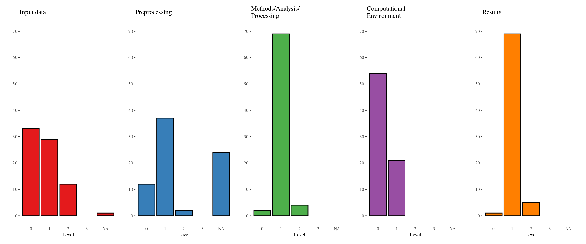

Figure: Alluvial diagramme of reproducibility assessment results across categories

This figure is based on package ggalluvial. It does not include the category preprocessing because it was discovered to be quite hard to assess, and subsequently has a large share of missing values. The figure also does not include any papers who have one or more categories as NA, as that means “not assessable”.

papers_wo_na_wo_prepr <- paper_evaluation_wo_conceptual %>%
  drop_na() %>%
  mutate_if(is.factor, forcats::fct_rev) %>%
  group_by(`input data`,
           `method/analysis/processing`,
           `computational environment`,
           results) %>%
  tally() %>%
  mutate(`Category levels (#)` = paste0(`input data`, " ",
                       `method/analysis/processing`, " ",
                       `computational environment`, " ",
                       results, " (", n, ")"))

fig_alluvial <- ggplot(data = papers_wo_na_wo_prepr,
       aes(axis1 = `input data`,
           axis2 = `method/analysis/processing`,
           axis3 = `computational environment`,
           axis4 = results,
           y = n)
       ) +
  ggplot2::scale_x_discrete(limits = c("Input Data",
                              "Methods/\nAnalysis/\nProcessing",
                              "Computational\nEnvironment",
                              "Results"),
                   expand = c(.1, 0)
                   ) +
  xlab("Category") +
  ylab("Number of papers") +
  ggplot2::scale_fill_manual(values = c(
    RColorBrewer::brewer.pal(9, "Set1"),            # colours from the other plots
    RColorBrewer::brewer.pal(4, "Dark2")[c(1,3,4)]) # manually chosen from another palette
    ) +
  ggalluvial::geom_alluvium(aes(fill = `Category levels (#)`), width = 1/3) +
  ggalluvial::geom_stratum(alpha = 1) +
  ggfittext::geom_fit_text(stat = "stratum", aes(label = after_stat(stratum)), min.size = 1) +
  ggthemes::theme_tufte()

fig_alluvial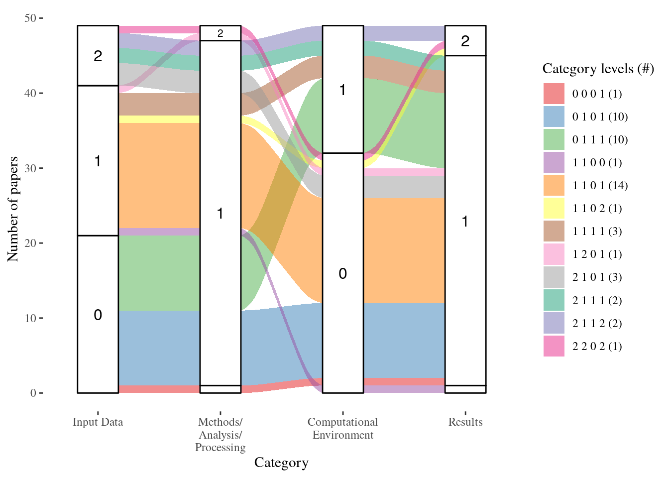

Table: Mean levels per criterion for non-conceptual papers

means <- lapply(evaldata_numeric %>%
                      select(all_of(categoryColumns)),
                    summary) %>%
    lapply(`[[`, "Mean") %>%
    as.data.frame()

kable(means,
      digits = 2,
      col.names = c("input data", "preproc.", "method/analysis/proc.", "comp. env.", "results"),
      caption = "Mean levels per criterion for non-conceptual papers") %>%
  kableExtra::kable_styling("striped", full_width = FALSE)

Mean levels per criterion for non-conceptual papers

input data	preproc.	method/analysis/proc.	comp. env.	results
0.72	0.8	1.03	0.28	1.05

Table: Mean levels averaged across criteria over time for non-conceptual papers

means_years <- evaldata_numeric %>%
  filter(`conceptual paper` == FALSE) %>%
  group_by(year) %>%
  summarise(mean = mean(c(`input data`, 
                          preprocessing, 
                          `method/analysis/processing`, 
                          `computational environment`, 
                          `results`),
                        na.rm = TRUE),
            `paper count` = n())

means_years_table <- means_years %>% 
        mutate(mean = round(mean, 2), 
               `paper count` = as.character(`paper count`)) %>%
        mutate(labels = str_c(year, " (n = ", `paper count`, ")")) %>%
        column_to_rownames("labels") %>%
        select(mean) %>%
        t()

kable(means_years_table,
      caption = "Summarised mean values over all criteria over time (non-conceptual papers)") %>%
  kableExtra::kable_styling("striped", full_width = TRUE)

Summarised mean values over all criteria over time (non-conceptual papers)

	2012 (n = 22)	2014 (n = 18)	2016 (n = 18)	2018 (n = 17)
mean	0.84	0.73	0.82	0.69

Figure: Mean reproducibility levels per category over time for non-conceptual papers

evaldata_years <- evaldata_numeric %>%
  filter(`conceptual paper` == FALSE) %>%
  group_by(year) %>%
  summarise(input = mean(`input data`, na.rm = TRUE),
         preprocessing = mean(preprocessing, na.rm = TRUE),
            method = mean(`method/analysis/processing`, na.rm = TRUE),
            environment = mean(`computational environment`, na.rm = TRUE),
            results = mean(results, na.rm = TRUE))
paper_count_years <- evaldata_numeric %>%
  filter(`conceptual paper` == FALSE) %>%
  group_by(year) %>%
  summarise(`paper count` = n())

evaldata_years_long <- melt(evaldata_years, id.vars = c("year"))
fig_mean_over_time <- ggplot(evaldata_years_long, aes(year, value)) +
  geom_bar(aes(fill = variable), position = "dodge", stat = "identity") +
  #geom_errorbar(stat = "summary", fun.data = "mean_sdl", 
  #                fun.args = list(mult = 1),
  #                position =  position_dodge(width = 0.9)) +
  ylab("mean value of criterion level") + 
  scale_x_continuous(breaks = evaldata_years$year,
                     labels = paste0(paper_count_years$year, 
                                     " (n=", 
                                     paper_count_years$`paper count`, 
                                     ")")) +
  scale_fill_brewer(palette = "Set1", name = "Category") +
  ggthemes::theme_tufte(base_size = 18) +
  theme(legend.position = c(0.15,0.75), 
        legend.text = element_text(size = 14)) +
  ylim(0, 3) +
  stat_summary(fun = mean, fun.min = mean, fun.max = mean, shape = "-", size = 2) +
  stat_summary(fun = mean, geom = "line", linetype = "dotted", mapping = aes(group = 1))

fig_mean_over_time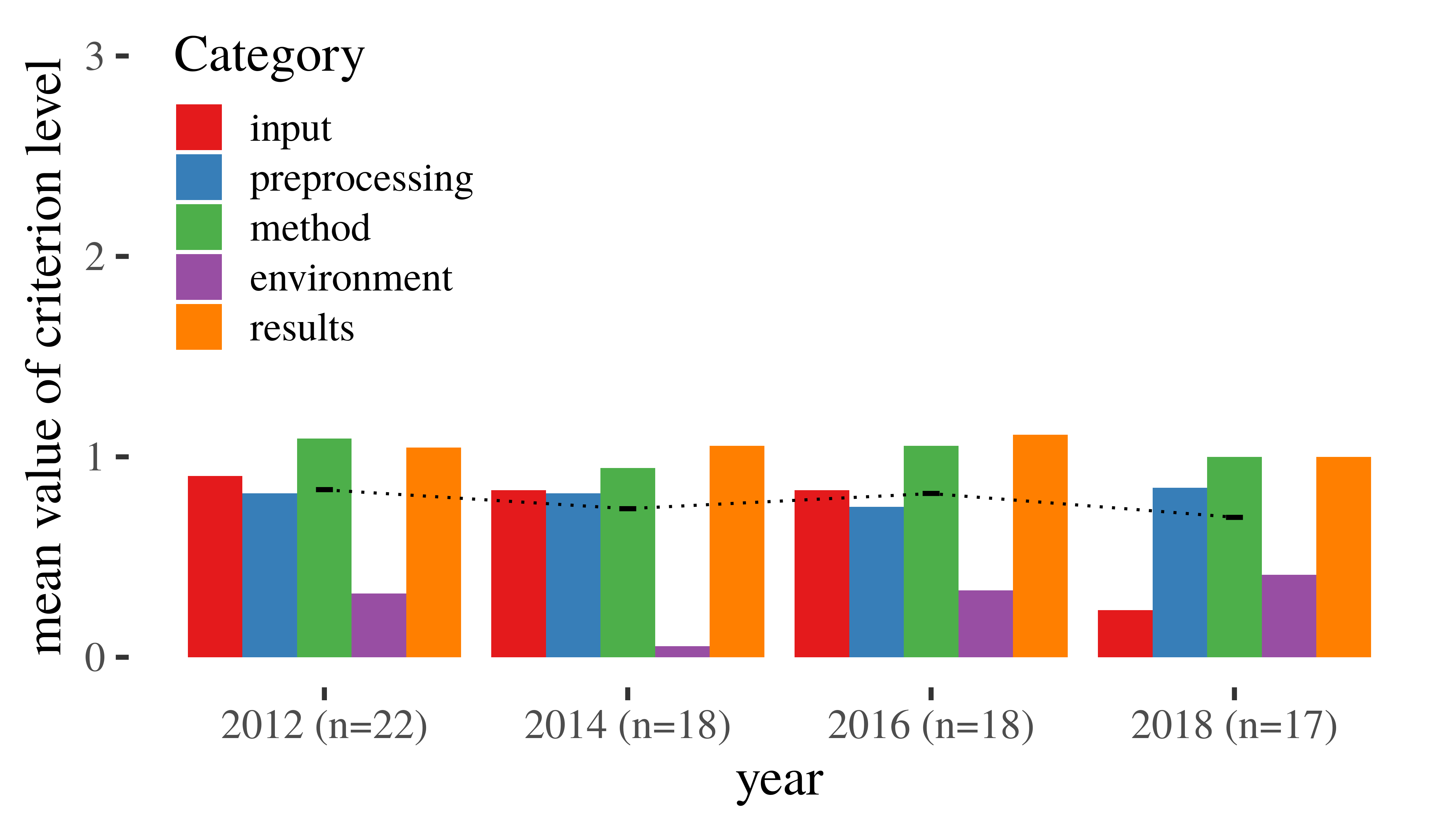

Colophon

This document is licensed under a Creative Commons Attribution 4.0 International License. All contained code is licensed under the Apache License 2.0. This document is versioned in a public git repository, https://github.com/nuest/reproducible-research-at-giscience, and archived on Zenodo at https://doi.org/10.5281/zenodo.4032875.

Runtime environment description:

## ─ Session info ───────────────────────────────────────────────────────────────────────────────────
##  setting  value                       
##  version  R version 3.6.3 (2020-02-29)
##  os       Debian GNU/Linux 10 (buster)
##  system   x86_64, linux-gnu           
##  ui       X11                         
##  language (EN)                        
##  collate  en_US.UTF-8                 
##  ctype    en_US.UTF-8                 
##  tz       Etc/UTC                     
##  date     2021-06-01                  
## 
## ─ Packages ───────────────────────────────────────────────────────────────────────────────────────
##  package       * version date       lib source                                  
##  assertthat      0.2.1   2019-03-21 [1] CRAN (R 3.6.3)                          
##  backports       1.1.6   2020-04-05 [1] CRAN (R 3.6.3)                          
##  base          * 3.6.3   2020-05-14 [2] local                                   
##  broom           0.5.6   2020-04-20 [1] CRAN (R 3.6.3)                          
##  callr           3.4.3   2020-03-28 [1] CRAN (R 3.6.3)                          
##  cellranger      1.1.0   2016-07-27 [1] CRAN (R 3.6.3)                          
##  cli             2.0.2   2020-02-28 [1] CRAN (R 3.6.3)                          
##  colorspace      1.4-1   2019-03-18 [1] CRAN (R 3.6.3)                          
##  compiler        3.6.3   2020-05-14 [2] local                                   
##  crayon          1.3.4   2017-09-16 [1] CRAN (R 3.6.3)                          
##  datasets      * 3.6.3   2020-05-14 [2] local                                   
##  DBI             1.1.0   2019-12-15 [1] CRAN (R 3.6.3)                          
##  dbplyr          1.4.3   2020-04-19 [1] CRAN (R 3.6.3)                          
##  desc            1.2.0   2018-05-01 [1] CRAN (R 3.6.3)                          
##  devtools        2.3.0   2020-04-10 [1] CRAN (R 3.6.3)                          
##  digest          0.6.25  2020-02-23 [1] CRAN (R 3.6.3)                          
##  dplyr         * 0.8.5   2020-03-07 [1] CRAN (R 3.6.3)                          
##  ellipsis        0.3.0   2019-09-20 [1] CRAN (R 3.6.3)                          
##  evaluate        0.14    2019-05-28 [1] CRAN (R 3.6.3)                          
##  fansi           0.4.1   2020-01-08 [1] CRAN (R 3.6.3)                          
##  farver          2.0.3   2020-01-16 [1] CRAN (R 3.6.3)                          
##  forcats       * 0.5.0   2020-03-01 [1] CRAN (R 3.6.3)                          
##  fs              1.4.1   2020-04-04 [1] CRAN (R 3.6.3)                          
##  generics        0.0.2   2018-11-29 [1] CRAN (R 3.6.3)                          
##  ggalluvial    * 0.11.3  2020-04-16 [1] CRAN (R 3.6.3)                          
##  ggfittext     * 0.8.1   2019-07-18 [1] CRAN (R 3.6.3)                          
##  ggplot2       * 3.3.0   2020-03-05 [1] CRAN (R 3.6.3)                          
##  ggthemes      * 4.2.0   2019-05-13 [1] CRAN (R 3.6.3)                          
##  glue            1.4.0   2020-04-03 [1] CRAN (R 3.6.3)                          
##  googlesheets4 * 0.1.1   2021-06-01 [1] Github (tidyverse/googlesheets4@ec3946b)
##  graphics      * 3.6.3   2020-05-14 [2] local                                   
##  grDevices     * 3.6.3   2020-05-14 [2] local                                   
##  grid          * 3.6.3   2020-05-14 [2] local                                   
##  gridBase      * 0.4-7   2014-02-24 [1] CRAN (R 3.6.3)                          
##  gridExtra     * 2.3     2017-09-09 [1] CRAN (R 3.6.3)                          
##  gtable          0.3.0   2019-03-25 [1] CRAN (R 3.6.3)                          
##  haven           2.2.0   2019-11-08 [1] CRAN (R 3.6.3)                          
##  here          * 0.1     2017-05-28 [1] CRAN (R 3.6.3)                          
##  highr           0.8     2019-03-20 [1] CRAN (R 3.6.3)                          
##  hms             0.5.3   2020-01-08 [1] CRAN (R 3.6.3)                          
##  htmltools       0.4.0   2019-10-04 [1] CRAN (R 3.6.3)                          
##  httr            1.4.1   2019-08-05 [1] CRAN (R 3.6.3)                          
##  huxtable      * 4.7.1   2020-01-08 [1] CRAN (R 3.6.3)                          
##  jsonlite        1.6.1   2020-02-02 [1] CRAN (R 3.6.3)                          
##  kableExtra    * 1.1.0   2019-03-16 [1] CRAN (R 3.6.3)                          
##  knitr         * 1.28    2020-02-06 [1] CRAN (R 3.6.3)                          
##  labeling        0.3     2014-08-23 [1] CRAN (R 3.6.3)                          
##  lattice         0.20-38 2018-11-04 [2] CRAN (R 3.6.3)                          
##  lifecycle       0.2.0   2020-03-06 [1] CRAN (R 3.6.3)                          
##  lubridate       1.7.8   2020-04-06 [1] CRAN (R 3.6.3)                          
##  magrittr        1.5     2014-11-22 [1] CRAN (R 3.6.3)                          
##  memoise         1.1.0   2017-04-21 [1] CRAN (R 3.6.3)                          
##  methods       * 3.6.3   2020-05-14 [2] local                                   
##  modelr          0.1.6   2020-02-22 [1] CRAN (R 3.6.3)                          
##  munsell         0.5.0   2018-06-12 [1] CRAN (R 3.6.3)                          
##  nlme            3.1-144 2020-02-06 [2] CRAN (R 3.6.3)                          
##  patchwork     * 1.1.0   2021-06-01 [1] Github (thomasp85/patchwork@48819a9)    
##  pillar          1.4.3   2019-12-20 [1] CRAN (R 3.6.3)                          
##  pkgbuild        1.0.6   2019-10-09 [1] CRAN (R 3.6.3)                          
##  pkgconfig       2.0.3   2019-09-22 [1] CRAN (R 3.6.3)                          
##  pkgload         1.0.2   2018-10-29 [1] CRAN (R 3.6.3)                          
##  plyr            1.8.6   2020-03-03 [1] CRAN (R 3.6.3)                          
##  prettyunits     1.1.1   2020-01-24 [1] CRAN (R 3.6.3)                          
##  processx        3.4.2   2020-02-09 [1] CRAN (R 3.6.3)                          
##  ps              1.3.2   2020-02-13 [1] CRAN (R 3.6.3)                          
##  purrr         * 0.3.4   2020-04-17 [1] CRAN (R 3.6.3)                          
##  R6              2.4.1   2019-11-12 [1] CRAN (R 3.6.3)                          
##  RColorBrewer    1.1-2   2014-12-07 [1] CRAN (R 3.6.3)                          
##  Rcpp            1.0.4.6 2020-04-09 [1] CRAN (R 3.6.3)                          
##  readr         * 1.3.1   2018-12-21 [1] CRAN (R 3.6.3)                          
##  readxl          1.3.1   2019-03-13 [1] CRAN (R 3.6.3)                          
##  remotes         2.1.1   2020-02-15 [1] CRAN (R 3.6.3)                          
##  reprex          0.3.0   2019-05-16 [1] CRAN (R 3.6.3)                          
##  reshape2      * 1.4.4   2020-04-09 [1] CRAN (R 3.6.3)                          
##  rlang           0.4.5   2020-03-01 [1] CRAN (R 3.6.3)                          
##  rmarkdown       2.5     2021-06-01 [1] Github (rstudio/rmarkdown@4ff2093)      
##  rprojroot       1.3-2   2018-01-03 [1] CRAN (R 3.6.3)                          
##  rstudioapi      0.11    2020-02-07 [1] CRAN (R 3.6.3)                          
##  rvest           0.3.5   2019-11-08 [1] CRAN (R 3.6.3)                          
##  scales          1.1.0   2019-11-18 [1] CRAN (R 3.6.3)                          
##  sessioninfo     1.1.1   2018-11-05 [1] CRAN (R 3.6.3)                          
##  stats         * 3.6.3   2020-05-14 [2] local                                   
##  stringi         1.4.6   2020-02-17 [1] CRAN (R 3.6.3)                          
##  stringr       * 1.4.0   2019-02-10 [1] CRAN (R 3.6.3)                          
##  testthat        2.3.2   2020-03-02 [1] CRAN (R 3.6.3)                          
##  tibble        * 3.0.1   2020-04-20 [1] CRAN (R 3.6.3)                          
##  tidyr         * 1.0.2   2020-01-24 [1] CRAN (R 3.6.3)                          
##  tidyselect      1.0.0   2020-01-27 [1] CRAN (R 3.6.3)                          
##  tidyverse     * 1.3.0   2019-11-21 [1] CRAN (R 3.6.3)                          
##  tools           3.6.3   2020-05-14 [2] local                                   
##  usethis         1.6.0   2020-04-09 [1] CRAN (R 3.6.3)                          
##  utils         * 3.6.3   2020-05-14 [2] local                                   
##  vctrs           0.2.4   2020-03-10 [1] CRAN (R 3.6.3)                          
##  viridisLite     0.3.0   2018-02-01 [1] CRAN (R 3.6.3)                          
##  webshot         0.5.2   2019-11-22 [1] CRAN (R 3.6.3)                          
##  withr           2.2.0   2020-04-20 [1] CRAN (R 3.6.3)                          
##  xfun            0.15    2021-06-01 [1] Github (yihui/xfun@06e86a6)             
##  xml2            1.3.2   2020-04-23 [1] CRAN (R 3.6.3)                          
##  yaml            2.2.1   2020-02-01 [1] CRAN (R 3.6.3)                          
## 
## [1] /usr/local/lib/R/site-library
## [2] /usr/local/lib/R/library